Numerical Analysis

Some of the numerical experiments are journaled here !

---

TOC:

• Using python for analysis of data acquired via a web-based database

---

Using python for analysis of data acquired via a web-based database

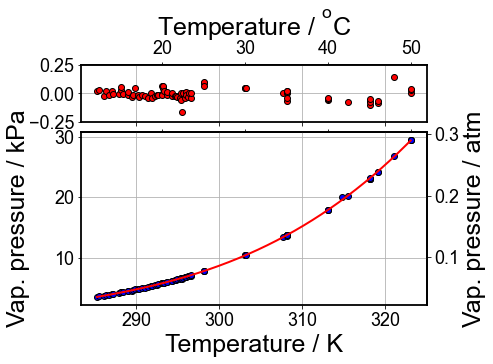
This is an example showing reading data from online database (formatted as an html page) via requests module in package and analyzed via numpy and scipy.

import requests
import pandas as pd
import numpy as np

# get data from webpage (here it is DDBST's dataset on ethanol)
url = 'http://www.ddbst.com/en/EED/PCP/VAP_C11.php'
html = requests.get(url).content
df_list = pd.read_html(html)
df = df_list[2]

print('\t\t---Extracted data---\n', df, '\n\t\t----------------------')

                ---Extracted data---
       T [K]   P [kPa]         State  Reference
0    273.15    1.5932  Vapor-Liquid          6
1    277.24    2.1065  Vapor-Liquid          1
2    277.24    2.1120  Vapor-Liquid          1
3    278.12    2.2330  Vapor-Liquid          1
4    278.12    2.2425  Vapor-Liquid          1
..      ...       ...           ...        ...
116  350.75   99.6980  Vapor-Liquid          2
117  350.85  100.0450  Vapor-Liquid          2
118  351.15  101.3250  Vapor-Liquid          2
119  351.25  101.3250  Vapor-Liquid          2
120  351.70  102.2200  Vapor-Liquid          6

[121 rows x 4 columns]
                ----------------------

# importing matplotlib for plotting !
import matplotlib.pyplot as plt
from matplotlib.pyplot import figure
import matplotlib.ticker as ticker
from matplotlib.offsetbox import AnchoredText

import matplotlib.font_manager as font_manager

plt.rcParams['lines.linewidth'] = 2 ;
plt.rc('axes', linewidth=1.80) ;
plt.rcParams["savefig.dpi"] = 340 ;
plt.rcParams.update({'font.size': 18}) ;
plt.rcParams["font.family"] = "Arial";
##############################################
def kelvin_to_C(x):
    return (x-273.15)

def kpa_to_atm(x):
    return x * (1 / 101.325)
##############################################

---

dfc = df

# trimmed
dfc.columns = [c.replace(' ', '_') for c in dfc.columns]
dfc.columns = [c.replace('[', '') for c in dfc.columns]
dfc.columns = [c.replace(']', '') for c in dfc.columns]

# filtering out data in the target region
dfc.T_K
dfc = dfc[dfc.T_K  < 325 ]
dfc = dfc[dfc.T_K  > 285 ]

temperature=dfc['T_K' ].values
kpa=dfc['P_kPa' ].values

print(temperature.shape, kpa.shape)

# 1D arrays of data
#    temperature
#    kpa

(80,) (80,)

# do a polynomial fit of the data points

z = np.polyfit(temperature, kpa, 3)
p = np.poly1d(z)
# z contains fit parameters
print('\t Fit coefficients : ', z)

# generate fit trace

fit_x = np.arange(temperature[0],temperature[-1], 0.05)

fit_y = p(fit_x)

diff = kpa - (p(temperature))

         Fit coefficients :  [ 1.76941577e-04 -1.46296686e-01  4.05062345e+01 -3.75390272e+03]

---

# Upper plot

fig1 = plt.figure(1, facecolor='white')

#plt.figure(facecolor='white')

frame1 = fig1.add_axes((.1, .1, .8, .6))

plt.plot(temperature, kpa ,'ob', markeredgecolor='black')
plt.plot(fit_x, fit_y,'-r')

#frame1.set_xticklabels([])
plt.grid()
ax = plt.gca()
secax = ax.secondary_xaxis('top', functions=(kelvin_to_C,kelvin_to_C))
secay = ax.secondary_yaxis('right', functions=(kpa_to_atm,kpa_to_atm))

plt.xlabel('Temperature / K', fontsize=25)
plt.ylabel('Vap. pressure / kPa', fontsize=25, labelpad=24)
#secax.set_xlabel('Temperature / $\mathregular{^{o}}$C', fontsize=25)
secay.set_ylabel('Vap. pressure / atm', fontsize=25)

spacing = 0.87980
fig1.subplots_adjust(left=spacing)

############################################

# Residual plot
difference = diff
frame2 = fig1.add_axes((.1,.734,.8,.2))
frame2.set_xticklabels([])
plt.plot(temperature ,difference,'or', markeredgecolor='black')
ax = plt.gca()
ax.set_ylim([-0.25, 0.25])

secax = ax.secondary_xaxis('top', functions=(kelvin_to_C,kelvin_to_C))
secax.set_xlabel('Temperature / $\mathregular{^{o}}$C', fontsize=25)
plt.grid()