Instrument or devices used to perform measurements are based on references against which different physical quantities are compared to. For example, a regular measurement tape is based on the definition of meter in the SI unit, and was transfered to the physical object, a piece of tape, while manufacturing by marking at specific intervals. This transfer of length (in this case for the measurement tape) might have been performed using a metallic bar of steel of length 1 meter, for example.
Similar analogies can be drawn up for various devices. Since, I work with optical devices and related electronics, I limit my discussion to few such examples.
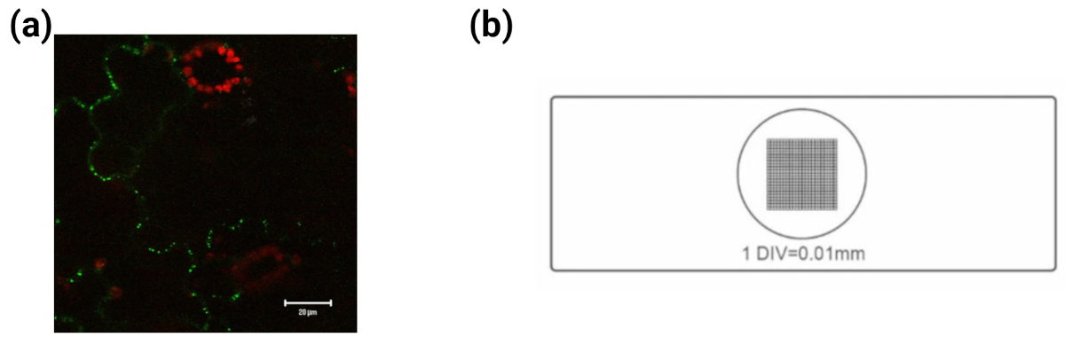
A microscope image (also called micrograph) has a bar which serves as a reference for length. The size of objects in the image are then obtained via a relative estimation. This bar is established via meaurement of grid of specified length (say a few \(\mu m\) ) on the same microscope and then transfer of length via counting the pixels from one point on the image grid to another. See images below for an example. The GFP image was adapted from wikepedia. }
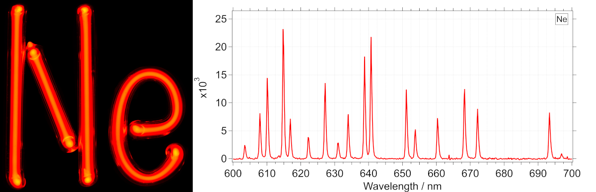
Wavelength positions on a typical uv-visibale absorption spectrometer are calibrated to reference emission lines from atoms. Atomic emission from different elements occur at very specfic and well defined wavelengths which vary to a very small extent on measurement conditions. One great example of this is emission from neon lamp. This looks orange in color to us, but has very well defined peaks but in the yellow and red region. See the spectrum below (only a part of the full emission spectrum is shown). This was measured on a cooled CCD detector with a grating based spectrograph using a cheap 110V mini neon lamp (~2022) as the light source.
The procedure goes as this : determine the position of a specific peak on the recorded spectra. Then assign this position on the spectra to a specific wavelength. Atomic emission lines serve as excellent reference for such work. If the measurement system consists of other moving parts, like a grating to disperse light, then grating center and motor position can be combined in an equation to also obtain the correct wavelength scale at different positions. This procedure forms the basis for essentially all wavelength (or wavenumber) calibration in spectroscopy. See spectral datasets below.
With this, I move to the discussion about calibation of Raman spectrometers. Raman spectra can be measured in two priniciple ways, in frequency domain and in the time-domain. In the frequency domain, Raman spectrometers sample the scattered photons which are spatially dispersed and their intensity is recorded via photon detector (for example, photodiode arrays, CCD, linear CCD array or CMOS sensors). In the time-domain measurements, Raman spectra is constructed via looking at oscillation of an optical signal at a frequency corresponding to the Raman transition and has a rather complex measurement techinique. However, most of the measurements are based on the frequency domain measurements based on one or more dispersive optical element(s), multi-channel detectors and a laser.
In the Raman spectrometer, light scattered by the molecules travels to the detector while passing through/by some optical components (for example, lens, mirrors, grating, etc..). In this process, the scattered light intensity is modulated by the non-uniform reflectance/transmission of the optical components. Reflectance and transmission of the optics are wavenumber dependent.
The net modulation to the light intensity, defined as \(M_{i}(\nu)\), over the studied spectral range can be expressed as product(s) of the wavenumber dependent performance of the \(i^{th}\) optical element as
\[M=\Pi c_{i} w_{i}(\nu)\]
Here, \(c_{i}\) is a coefficient and \(w_{i}(\nu)\) is the wavenumber dependent transmission (or reflectance) of the \(i^{th}\) optical component. However, in most cases, determining the individual performance of each optical element is a cumbersome task and the approach for accounting the effect of each optics individually is rather difficult. Spatial variations can’t be accounted for in such an approach.
There have been different ways to account for this modulation of the recorded spectrum. A bried summary is as follows:
Using fluorescence based standards : Broadband fluorescence has been used for a long time due to the simplicity of the measurement setup and the advent of solid state samples. In this regard, the early samples were fluorophores dissolved in a solvent, for example, quinine, etc.. Disadvantages are several: the stability of the sample, concentration dependence of the fluorophore if a liquid solution is used and obtaining a reliable polarization dependence of the spectrometer.
Using broad-band emission from lamps : Heated filament lamps can be assumed to be black-body emittor with emission profile explained by equation providing emission intensity for a given wavelength. This known profile was used together with the temperature of the lamp to derive the relative sensitivity. Disadvantage is that the temperature of the lamp has to be known. Further, information about polarization dependent sensitivity is difficult to be derived from this approach. One may assume that the emission is purely random, and a diffuser may be used to account for this.
Using Raman intensities themselves : Raman intensities give another way to extract out the sensitivity information from recorded spectra. However, the peaks to be used for this purpose must be well defined, i.e. narrow and negligible baseline, so as to help in accurate band area determination. This puts certain limitations about what kind of Raman transitions can be used for the purpose. Rotational and ro-vibrational transitions are one such candidate. Usage of molecular hydrogen and nitrogen have been demonstrated for this purpose.
In general, the calibration work of Raman spectrometer has been well described in the popular textbook by Prof. Richard McCreery (Raman Spectroscopy for Chemical Analysis), with the exception discussion on using Raman spectra for intensity calibration work. Standard tungsten lamps can be used for preliminary calibration as discussed in this (: technicalreport(PDF) ).
In my study performed at NYCU, the broad-band emission from tungsten lamp and analysis of Raman spectra of a few gases (rotational and ro-vibrational transitions) were used to obtain the sensitivity information of the Raman spectrometer. Thus, I limit the focus to determine the relative form of \(M_{i}(\nu)\), from experimental data. By relative form, it is meant that \(M_{i}(\nu)\) is normalized to unity within the studied spectral range. If \(M_{i}(\nu)\) is known, then we can correct the observed intensities in the Raman spectrum by dividing those by \(M_{i}(\nu)\).
In my work, we assume \(M_{i}(\nu) = \frac{C_{0}}{C_{1}C_{2}}\), thus a product of three functions. The wavenumber dependence in not explicitly stated when \(C_{0}\), \(C_{1}\) and \(C_{2}\) are discussed in the following text, and the three contributions are determined in a two steps in my proposed analysis.
In the first step, \(M_{i}(\nu) = \frac{C_{0}}{C_{1}}\) correction is determined using the wavenumber axis and the spectrum of a broad band white light source. Refer to this jupyter notebook on github.
Next, \(M_{i}(\nu) = C_{2}\) is determined from the observed Raman intensities, where the reference or true intensities are known or can be computed. This can be done using (i) pure-rotational Raman bands of molecular hydrogen and isotopologues, (ii) vibration-rotation Raman bands of the same gases, and (iii) vibrational Raman bands of some liquids.
The multiplicative correction to the Raman spectrum is then : \(M_{i}(\nu) = \frac{C_{0}}{C_{1}C_{2}}\)
The present scheme is a multi-step procedure based on following three steps:
For the non-linear sampling of photons in the wavenumber scale, \(M_{i}(\nu) = C_{0}\)
For the channel-to-channel variation in the sensitivity of the spectrometer, \(M_{i}(\nu) = {C_{1}}\)
and lastly, final correction derived from Raman spectroscopic intensities, \(M_{i}(\nu) = {C_{2}}\) :
In order to determine the final correction \(M_{i}(\nu) = C_{2}\), the relative band intensities between all pairs of bands are analyzed simultaneously by a comparison with the analogous reference intensities. Least squares minimization is used to determine the coefficients of a polynomial used to model the wavelength-dependent sensitivity representing the \(M_{i}(\nu) = C_{2}\) correction.
For more details refer to the following work, discussing the fingerprint region (article 1), and then discussing the high-wavenumber region (article 2). PDFs are available on request. These works are provided with computer codes and detailed supporting information for quick applications in research.
This lamp commonly used in homes and office spaces gives pleasant white light, which however is a combination of emission from Hg ions and fluorescence from phosphor coating. The phosphor coating luminesces due to the UV emitted by the Hg ions.
Wavenumber calibration data for Raman spectroscopy
Reference data on pure organic liquids for wavenumber calibration
Raman spectrometer calibrated using rotational Raman lines of gases was used to obtain this dataset. (see https://doi.org/10.1002/jrs.5955)
Carbon tetrachloride (CCl4)
Mode
ν (cm⁻¹)
Δν
ρ
Δρ
v₂ (e)
218.1
0.6
0.759
0.012
v₄ (f₂)
313.9
0.6
0.755
0.011
v₁ (a₁)
460.2
0.6
0.028
0.012
v₃ / (v₁+v₄) (f₂)
759.4
0.8
0.759
0.020
v₃ / (v₁+v₄) (f₂)
789.6
0.8
0.754
0.017
Cyclohexane (C6H12)
Mode
ν (cm⁻¹)
Δν
ρ
Δρ
v₆ (a₁g), CCC deform + CC torsion
383.1
0.6
0.146
0.010
v₂₄ (e_g), CCC deform + CC torsion
426.0
0.6
0.748
0.018
v₅ (a₁g), CC stretch
801.3
0.5
0.088
0.003
v₂₂ (e_g), CC stretch
1027.7
0.5
0.751
0.021
v₄ (a₁g), CH₂ rock
1157.3
0.6
0.282
0.010
v₂₁ (e_g), CH₂ twist
1266.1
0.6
0.759
0.021
v₂₀ (e_g), CH₂ wag
1346.5
0.7
0.748
0.030
v₁₉ (e_g), CH₂ scissoring
1443.7
0.8
0.746
0.019
Benzene (C6H6)
Mode
ν (cm⁻¹)
Δν
ρ
Δρ
Ring deform (v18)
607.0
0.6
0.749
0.021
Ring stretch (v2)
992.3
0.5
0.055
0.005
CH bend (v17)
1176.5
0.6
0.759
0.029
Fermi res. (v16, v2+v18)
1585.5
0.7
0.752
0.036
v2 + v18
1606.7
0.7
0.770
0.051
Toluene (C6H5–CH3)
Mode
ν (cm⁻¹)
Δν
ρ
Δρ
v₁₃ (a₁)
521.2
0.5
0.306
0.005
v₁₂ (a₁)
786.0
0.5
0.033
0.003
v₁₁ (a₁)
1003.3
0.5
0.032
0.003
v₁₀ (a₁)
1030.3
0.6
0.076
0.004
v₃₄ (b₂)
1155.6
0.9
0.690
0.021
v₉ (a₁)
1179.1
0.9
0.759
0.027
v₈ (a₁)
1210.0
0.6
0.057
0.003
Benzonitrile (C6H5–CN)
Mode
ν (cm⁻¹)
Δν
ρ
Δρ
Ring deform + CC stretch (v12)
460.8
0.6
0.183
0.009
CCN linear bend + CC wag (v20)
548.6
0.6
0.693
0.018
Ring deform (v31)
624.7
0.7
0.699
0.023
Ring deform (v10)
1000.7
0.5
0.051
0.006
C–C stretch (v9)
1026.6
0.6
0.043
0.005
C–C stretch (v5)
1599.0
0.5
0.566
0.030
Alignment of polarizer/analyzer for Raman spectroscopy
Polarization resolved Raman spectroscopic measurements require arrangement of a linear polarizer for the excitation laser (if not linearly polarized), and another linear polarizer (used as an analyzer) in the collection path. In this situation, one needs to find the orthogonal angular position of the analyzer relative to the incident laser polarization.
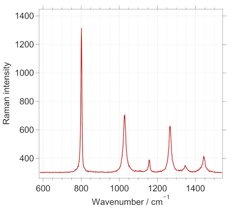
This note deals with the experimental determination of the angle on the analyzer. For this purpose, depolarized Raman signal is best suited, and in this page, the use of Raman peaks of cyclohexane is demonstrated for the purpose. The following figure shows the Raman spectrum of cyclohexane liquid.
One can simply compare the polarized and depolarized peaks in terms of their intensity ratios to determine when the analyzer is orthogonal to to the polarizer.
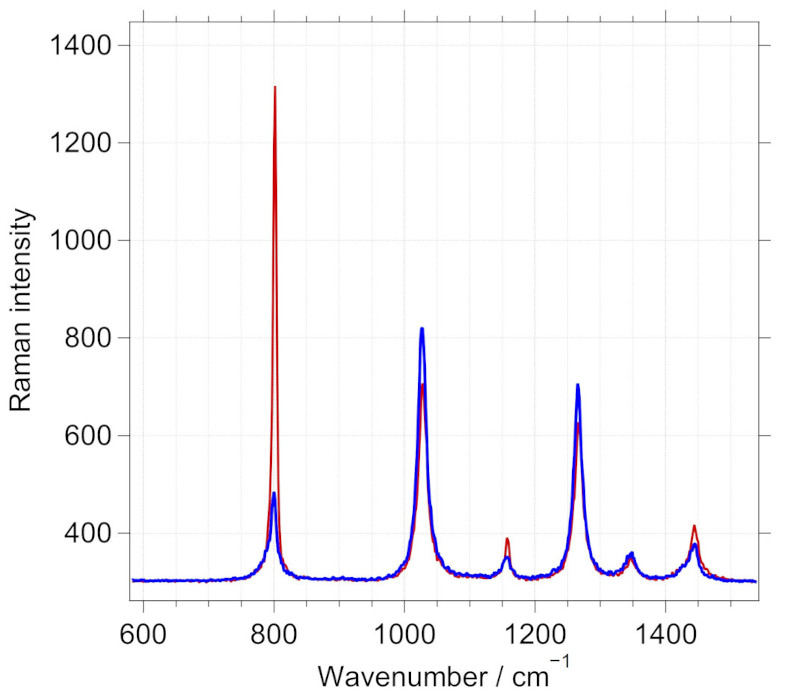
For this purpose, a series of measurements are performed while changing the angular position of the analyzer. When the analyzer only allows the depolarized signal to pass through, the polarized peaks are minimized. This is exemplified in the next figure.
Raman spectrum of cyclohexane in the fingerprint region with analyzer close to the orthogonal position is shown in blue. A marked decrease in the polarized Raman peak observed at 801.3 \(cm^{-1}\) is observed here for the blue spectrum.
Thus, intensity ratio of the polarized to depolarized peak as a function of the analyzer angle would give us information where the orthogonal position is. This is shown for one such performed measurement.
Raman intensity ratio of the polarized 801.3 peak to the depolarized 1027 peak is plotted as a function of the angle of the analyzer. The position of the center of the minima shows the position, in this case close to 64 \(^{\circ}\) where the analyzer is orthogonal to the linear incident polarization (or the polarizer for the incident beam, if used).
The oberved intensity ratios (in red color) were fit to a function of the form, \(f(x) = ( ((x-a_{0})^{2})*a_{1}) + a_{2}\), where \(a_{0}\) describes the center of the minima. The fit is shown in blue color. Least-squares fitting provides the most optimal values.